Mathematica Programming » Performance Tuning
Mathematica is what is often called a high-level programming language, because when you are writing programs, you don't need to worry about how the computer is doing its job. This provides notable gains in simplicity and scalability of large programs, but it comes at the cost of the speed and efficiency of low-level computations.
Basics of Compilation
To get around this Mathematica provides the function Compile which will generate a low-level function that we can then apply with fantastic results. For example, in the section on Nest I provided a random vector generator:
This creates a compiled function that will perform the task at hand, in this case taking a vector of Real numbers and returning a vector. Just so we can see the difference let's create the same function, uncompiled and compare the two:
 randomVector=
  Compile[{{mag,_Real}},
    mag*(#/Norm[#])&@RandomReal[{-1,1},3]
    ]
 randomVectorU=
  Function[mag,
    mag*Normalize@RandomReal[{-1,1},3]
    ];
Then we'll compare them using a little timing function:
 compareTiming[f1_,f2_,its_:1]:=
  With[{
      tf1=First@AbsoluteTiming[Do[f1,its]],tf2=First@AbsoluteTiming[Do[f2,its]]},
    (tf2-tf1)/Max@{tf1,tf2}
    ];
compareTiming~SetAttributes~HoldAll;

compareTiming[
  randomVector[1],
  randomVectorU[1],
  10^6
  ]
0.5244177474084153`
So we get a 52% speed boost from essentially just changing Function to Compile on the simplest function imaginable. If we had a more involved function the speed boost would likely be even larger. But since it's so simple we can easily dissect what is giving the speed boost:
Analyzing Compile
We'll build from the bottom up:
 randomReal3=Compile[{},RandomReal[{-1,1},3]];
randomReal3U=Function[RandomReal[{-1,1},3]];
compareTiming[randomReal3[], randomReal3U[],10^6]
0.4059389866935647`
This alone is 40% faster! Of course when we know how many vectors we'll need ahead of time the fastest thing is to use the syntax RandomReal[range,{count,3}] which can, for example, generate 10^8 random vectors in a fraction of a second, which is much, much faster than our compiled form:
compareTiming[Do[randomReal3[], 10^7], RandomReal[{-1, 1}, {3, 10^7}]]
-0.9477078222470973`
Ignoring the correct way to do this, though, and considering out surprising result, this is likely an artifact of type-checking in the compiled function that has to be performed at each call in the uncompiled one.
When we add our normalization now:
 randomVectorNoMag=
  Compile[{},
    (#/Norm[#]&)@RandomReal[{-1,1},3]
    ];
randomVectorNoMagU=
  Function[
    Normalize@RandomReal[{-1,1},3]
    ];
compareTiming[randomVectorNoMag[], randomVectorNoMagU[], 10^6]
0.4923576135986387`
Now we're a full 50% faster than we were (that this is greater than our original 40 is likely just a lack of consistency between runs).
Note that I'm in the CompiledFunction I'm not using Normalize . This is because Normalize cannot be directly compiled.
We can see this by looking at the intermediate representation generated when we use it:
 <<CompiledFunctionTools`
CompilePrint@
  Compile[{},
    Normalize@RandomReal[{-1,1}, 3]
    ]//Snippet[#, -5]&
 1 R0 = I1
2 R1 = I2
3 T(R1)1 = RandomReals[ R0, R1, T(I1)0]]
4 T(R1)2 = MainEvaluate[ Hold[Normalize][ T(R1)1]]
5 Return
The call to "MainEvaluate" means that the compiled function couldn't handle this and thus it returns the value to the main evaluator to process.
Drastic Examples
The previous case was simple so that it could easily be analyzed, but for more complicated cases we can much bigger gains. Consider the primary gradient function we used in the section on FixedPoint :
 gradient=
  Compile[{{pos,_Real,1}},
    {
      Piecewise[{
          {Sqrt@-(#+2),#<-3},
          {(-(#+2)^3),-3<#<0},
          {-((#-2)^3),0<=#<3},
          {-Sqrt@(#-2),3<=#}
          },#]&@pos[[1]],
      Piecewise[{
          {Sqrt@-(#),#<-1},
          {(-(#)^3),-1<=#<=1},
          {-Sqrt@(#),1<=#}
          },#]&@pos[[2]],
      Piecewise[{
          {Sqrt@-(#),#<-1},
          {(-(#)^3),-1<=#<=1},
          {-Sqrt@(#),1<=#}
          },#]&@pos[[3]]
      }
    ];
And then consider its uncompiled cousin:
 gradientU=
  Function[pos,
    {
      Piecewise[{
          {Sqrt@-(#+2),#<-3},
          {(-(#+2)^3),-3<#<0},
          {-((#-2)^3),0<=#<3},
          {-Sqrt@(#-2),3<=#}
          },#]&@pos[[1]],
      Piecewise[{
          {Sqrt@-(#),#<-1},
          {(-(#)^3),-1<=#<=1},
          {-Sqrt@(#),1<=#}
          },#]&@pos[[2]],
      Piecewise[{
          {Sqrt@-(#),#<-1},
          {(-(#)^3),-1<=#<=1},
          {-Sqrt@(#),1<=#}
          },#]&@pos[[3]]
      }
    ];

With[{grid=RandomReal[{-5,5},{10^5,3}]},
  compareTiming[
    gradient@g,
    gradientU@g,
    {g,grid}]
  ]
0.8961919038258733`
So the simple application of Compile provides a 90% speed boost.
As another example, one can implement numerical integration of a volume over a surface via:
 compDotCross=
  Compile[{{coords, _Real, 2}, {abc,_Integer,1}},
    coords[[ abc[[1]] ]].
    Cross[coords[[ abc[[2]] ]], coords[[ abc[[3]] ]]]
    ];
vol[s_?RegionQ]:=
  With[
    {coords = MeshCoordinates[s]},
    (MeshCells[s, 2]/.Polygon[g_List] :> compDotCross[coords, g])
    //Total
    ]/6
then get an interesting surface:
 surf=
  RegionUnion@@
    With[
      {
        graphics=
          FirstCase[
            ChemicalData["Caffeine", "SpaceFillingMoleculePlot"],
            _GraphicsComplex,
             None,
            ∞
            ]
        },
      Cases[
        graphics[[2]],
        Sphere[s_, r_]:>Ball[graphics[[1, s]], r]
        ]
      ]//BoundaryDiscretizeRegion[#, MaxCellMeasure->{1->20}]&
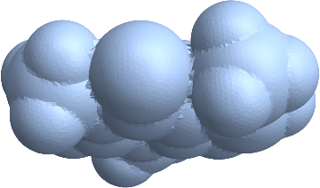
And compute its volume:
vol@surf//RepeatedTiming
 {0.0989207000000000003`2.,1.6728430521905467`*^8}

Volume@surf//RepeatedTiming
{0.0010948070175438598`2.,1.6728430521905503`*^8}
Our little compiled implementation is much slower than the built-in implementation, of course, but it's still incredibly fast for the level of mesh refinement.
Personally, I this it for computing atomic orbital volumes derived from orbital contour plots.
Lets then to a version without the compiled dot-cross:
 uncompDotCross=
  Function[{coords, abc},
    coords[[ abc[[1]] ]].
    Cross[coords[[ abc[[2]] ]], coords[[ abc[[3]] ]]]
    ];
volU[s_?RegionQ]:=
  With[
    {coords = MeshCoordinates[s]},
    (MeshCells[s, 2]/.Polygon[g_List] :> uncompDotCross[coords, g])
    //Total
    ]/6

compareTiming[vol@surf, volU@surf]
0.9539375762845481`
Ours is a whopping 95% faster. As the surface refinement increases this can be the difference between a function being nearly instantaneous versus a major speed bump in the research process.
We can also compare the version where we compile to C (i.e. we use CompilationTarget->"C"
 compDotCross=
  Compile[{{coords, _Real, 2}, {abc,_Integer,1}},
    coords[[ abc[[1]] ]].
    Cross[coords[[ abc[[2]] ]], coords[[ abc[[3]] ]]],
    CompilationTarget->"C"
    ];
volC[s_?RegionQ]:=
  With[
    {coords = MeshCoordinates[s]},
    With[{compiledDotCross=compDotCross},
      (MeshCells[s, 2]/.Polygon[g_List] :> compiledDotCross[coords, g])
      //Total
      ]/6
    ]

compareTiming[volC@surf, vol@surf]
0.13463908089141324`
And simply compiling to C made the function 13% faster. More performance can be eked but by using the difference RuntimeOptions and things.
Using Compile
It's often unclear whether a given function can be compiled or not, but happily Mathematica provides all of the possible compilable functions in Compile`CompilerFunctions . We can use this to make a compileableQ type function:
 compilableQ[f_]:=
MemberQ[Compile`CompilerFunctions[], f]
For example, we can see that, say, RandomVariate is compilable:
compilableQ@RandomVariate
True
Alternatively we can figure out which Random⋆ functions are compilable:
 compilableSelect[p_]:=
Select[Compile`CompilerFunctions[], StringMatchQ[ToString@#,p]&]

compilableSelect@"Random*"
{RandomChoice,RandomSample,RandomInteger,RandomVariate,RandomComplex,RandomReal,Random}
Once we have that, Compile has a very simple call structure that is similar to Module :
 Compile[
  {
    {var1,type1,arraySize1},
    {var2,type2,arraySize2},
    ...
    },
  expression,
  ops
  ]
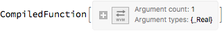
This will generate a CompiledFunction which is just a function in either Mathematica byte code or C byte code, as specified by the CompilationTarget option. In most cases Mathematica byte code is more than fast enough, but there are cases where the C code is a significantly better choice.