‌

Built-in Data and Units

Mathematica provides access to a lot of data, most useful for chemistry is the built-in chemical, element, and isotope data and the physical constants it knows about

ElementData

ElementData is a function that gets data on an element from Mathematica's built in servers. Here's a way to get the atomic number of an element:

 ElementData["W", "AtomicNumber"]

 74

We can also get things with units attached as a Quantity object:

 ElementData["H", "AtomicMass"]

 1.00794u

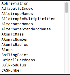
Here is the full list of properties to query for each element:

 Pane[Column@ElementData["Properties"],
  ImageSize->{Automatic,{150,250}},
  Scrollbars->{False, True},
  AppearanceElements->None
  ]//Framed[#,Background->White]&

And here is a function to apply that to a given element

 elementProperties[el_]:=
  Pane[Column@Table[With[{p=p},
    Button[Mouseover[p,Style[p,Orange]],
      With[{next=NextCell[EvaluationCell[]],cell=Cell[BoxData@ToBoxes@(p->ElementData[el,p]),"Output",
          CellFrame->{{0,0},{1,5}},
          CellMargins->With[{m=CellMargins/.Options[EvaluationCell[],CellMargins]},
            ReplacePart[m,{2,2}->0]
            ],
          "CellFrameStyle"->{{None,None},{Black,GrayLevel[.8]}}]},
      If[next=!=None&&GeneratedCell/.Options[next,GeneratedCell]//TrueQ,
        NotebookWrite[next,cell],
        CellPrint@cell
        ]],
      Appearance->"Frameless",
      Method->"Queued",
      BaseStyle->"Hyperlink"]
    ],
  {p,ElementData@"Properties"}],
  ImageSize->{Full,{150,250}},
  Scrollbars->{False, True},
  AppearanceElements->None
  ]//Framed[#,Background->White]&

elementProperties["H"]

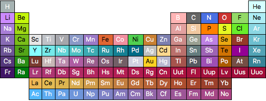
A list of all the elements can be generated via ElementData[] and I used that to generate a template for a periodic table. So finally here is a function that uses this template and the previously defined function to get all the possible information from ElementData.

 periodicTable[]:=
  With[{dlen=10,slen=2,plen=6},
    {
      {"H"}~Join~ConstantArray[Null,dlen+plen]~Join~{"He"},
      {"Li","Be"}~Join~ConstantArray[Null,dlen]~Join~{"B","C","N","O","F","Ne"},
      {"Na","Mg"}~Join~ConstantArray[Null,dlen]~Join~{"Al","Si","P","S","Cl","Ar"},
      {"K","Ca","Sc","Ti","V","Cr","Mn","Fe","Co","Ni","Cu","Zn","Ga","Ge","As","Se","Br","Kr"},
      {"Rb","Sr","Y","Zr","Nb","Mo","Tc","Ru","Rh","Pd","Ag","Cd","In","Sn","Sb","Te","I","Xe"},
      {"Cs","Ba","Lu","Hf","Ta","W","Re","Os","Ir","Pt","Au","Hg","Tl","Pb","Bi","Po","At","Rn"},
      {"Fr","Ra","Lr","Rf","Db","Sg","Bh","Hs","Mt","Ds","Rg","Cn","Uut","Fl","Uup","Lv","Uus","Uuo"},
      ConstantArray[Null,slen]~Join~{"La","Ce","Pr","Nd","Pm","Sm","Eu","Gd","Tb","Dy","Ho","Er","Tm","Yb"},
      ConstantArray[Null,slen]~Join~{"Ac","Th","Pa","U","Np","Pu","Am","Cm","Bk","Cf","Es","Fm","Md","No"}
      }
    ]//Grid[#,Alignment->Center]&//ReplaceAll[#,{
      e_String:>With[{color=Replace[
          ColorData["Atoms"][e],
          Except[_RGBColor]->Gray]},
      Item[
        Button[
          Mouseover[Style[e,If[ColorDistance[Black,color]<.9//TrueQ,
            White,
            Black]],
          Style[e,Orange]],CreateDocument[{Cell[BoxData@ToBoxes@elementProperties@e,"Output"],
            Cell["",GeneratedCell->True]},
          Background->color,
          WindowTitle->Capitalize@ElementData[e,"Name"],
          WindowSize->{400,365},
          StyleDefinitions->Notebook@{
            Cell[StyleData[StyleDefinitions->"Default.nb"]],
            Cell[StyleData@"Output",
              Background->White,
              CellMargins->{{10, 0}, {0, 10}}]
            },
          WindowElements->{},
          WindowFrameElements->{"CloseBox","ZoomBox","MinimizeBox"},
          Saveable->False,
          ScrollingOptions->{"VerticalScrollRange"->FitAll}],
        Appearance->"Frameless"
        ],
      Background->color,
      Frame->True
      ]
    ]
  }]&//Deploy

Since this function calls elementProperties be sure to evaluate the definition for elementProperties before evaluating the following.

 periodicTable[]

IsotopeData

IsotopeData is similar to ElementData except one supplies an isotope instead. Known isotopes for a given element can be gotten via the following function

 knownIsotopes[element_]:=
  Table[element<>ToString@i,{i,ElementData[element,"KnownIsotopes"]}]

knownIsotopes@"H"

 {"H1","H2","H3","H4","H5","H6","H7"}

We can similarly get all the properties for an isotope in the same way as for an element:

 isotopeProperties[iso_]:=
Pane[Column@Table[With[{p=p},
  Button[Mouseover[p,Style[p,Orange]],
    With[{next=NextCell[EvaluationCell[]],cell=Cell[BoxData@ToBoxes@(p->IsotopeData[iso,p]),"Output",
        CellFrame->{{0,0},{1,5}},
        CellMargins->With[{m=CellMargins/.Options[EvaluationCell[],CellMargins]},
          ReplacePart[m,{2,2}->0]
          ],
        "CellFrameStyle"->{{None,None},{Black,GrayLevel[.8]}}]},
    If[next=!=None&&GeneratedCell/.Options[next,GeneratedCell]//TrueQ,
      NotebookWrite[next,cell],
      CellPrint@cell
      ]],
    Appearance->"Frameless",
    Method->"Queued",
    BaseStyle->"Hyperlink"]
  ],
{p,IsotopeData@"Properties"}],
ImageSize->{Full,{150,250}},
Scrollbars->{False, True},
AppearanceElements->None
]//Framed[#,Background->White]&

isotopeProperties["H2"]

ChemicalData

The final useful data set is the built in ChemicalData which can return properties of chemicals generally. At this point it should be clear how it works, but it's worth pointing out that the list of all the known chemicals can take a long time to load so only call ChemicalData without any arguments if you're sure your internet connection is good and your computer can handle the load.

Quantity

The interface to the units Mathematica knows about is called Quantity

This was used previously to get the value of the molar gas constant, but there is a host of useful units built in. For example let's convert between a wavelength and a frequency for electromagnetic radiation:

Let's start out with green light. Let's find a frequency that works using Mathematica's built-in ColorData , which knows the frequencies of the visible spectrum.

Unfortunately this can only convert from a wavelength to a color, but we can write a function to get close to the appropriate wavelength, knowing that in Mathematica a color is just RGBColor[redPercentage,greenPercentage,bluePercentage] .

First we write a distance function:

 rgbDistance[color1_,color2_]:=(color1-color2)/.RGBColor->List//Norm;

Then we get the minimum distance to our given color of all the wavelengths in the visible spectrum: (for convenience I use a more complicated function declaration syntax, which is explained later)

 closestWavelength[
  color_,
  range:_List:ColorData["VisibleSpectrum"][[3]],
  step:_?NumericQ:1
  ]:=Quantity[
  First@MinimalBy[
    Range@@Append[range,step],
    rgbDistance[color,ColorData["VisibleSpectrum"][#]]&],
  "Nanometers"]
λ=closestWavelength[Green]

 541nm

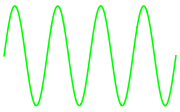
We can check that this is in fact a wavelength that corresponds to green light:

 Plot[Sin[4x],{x,-π,π},
  Axes->False,
  PlotStyle->ColorData["VisibleSpectrum"][QuantityMagnitude@λ],
  ImageSize->Small
  ]

Then we'll convert this to a frequency by recalling c=λν

 ν=UnitConvert[Quantity[1.,"SpeedOfLight"]/λ,"Hz"]

 5.54145*10^14Hz

Another place this is incredibly useful is for simple unit conversion problems, such as a classic PV=nRT application. Here's a sample problem I found online:

Determine the volume of occupied by 2.34 grams of carbon dioxide gas at STP.

We can solve this trivially using this built-in data:

 n = Quantity[2.34, "Grams"]/ChemicalData["CarbonDioxide", "MolarMass"];
P = Quantity[1, "Atmospheres"];
T = Quantity[273, "Kelvins"];
R = Quantity["MolarGasConstant"];
V = UnitConvert[n*R*T/P, "Liters"]

 1.1911L

It performs all the tedious conversions and has all the data. All we need to do is supply the formula.