‌

Packed Arrays

Mathematica has a wide variety of low-level optimizations that we never run into in our high-level usage. One of the most useful of these is the concept of the PackedArray .

These are efficiently stored arrays of a single type of object that perform much faster on many simple numerical manipulations than their "unpacked" companions.

Most internal functions that return arrays will return them in packed form. We can check that an array is packed with Developer`PackedArrayQ :

 reals = RandomReal[{-1, 1}, {1000, 1000}];
Developer`PackedArrayQ@reals

 True

The memory footprint of these is much lower than standard arrays:

 ureals=Developer`FromPackedArray@reals;
Developer`PackedArrayQ@ureals
ByteCount@reals
ByteCount@ureals

 False

 8000152

 24208200

And operations that can return a packed array are faster than their unpacked variants:

 1+reals//RepeatedTiming//First
1+ureals//RepeatedTiming//First

 0.0024543400000000002`3.

 0.0099898333333333315`2.

Unpacking

The biggest thing to worry about with packed arrays is the time/memory footprint that occurs when a packed array must be unpacked to be processed by a function that can't handle it in packed form.

For instance the function Chop necessarily unpacks as it replaces the Real number 0. with the Integer number 0 . This means Chop will actually be slower on a packed array:

 Chop@reals//RepeatedTiming//First
Chop@ureals//RepeatedTiming//First

 0.1129493750000000046`2.

 0.052316666666666671`2.

But if we use a function that can leverage the packing of the array it will be faster. For instance, let's look at the Real variant of Chop , a function called Threshold :

 Threshold@reals//RepeatedTiming//First
Threshold@ureals//RepeatedTiming//First

 0.0030930624999999999`2.

 0.0107768695652173899`2.

The packed version is much faster now.

‌

RawArray

The RawArray is a relatively new addition to the language. It works rather like PackedArray in its requirement ot use a single type of object in it, but is a fundamentally different object.

It's main benefit is how little memory it consumes:

 reals//ByteCount

 8000152

If we use a 64-bit real we get similar memory consumption to the packed array:

 raw64=RawArray["Real64", reals];
raw64//ByteCount

 8000096

But we can specify that it out to use half as many bytes, as the memory usage will drop correspondingly:

 raw32=RawArray["Real32", reals];
raw32//ByteCount

 4000096

These can also be used more effectively via Library Link but we won't get into that now. For many data-intensive custom Import formats RawArray can help cut down on the memory consumption, particularly where some large portions of the data may not be immediately useful.

‌

SparseArray

We won't discuss SparseArray much, as the sparse array is a well-known concept especially in numerical linear algebra.

It is worth keeping in mind, though, for places where one has highly sparse data. One classic place this can show up is in quantum mechanical calculations in a direct-product basis constructed from orthonormal bases. Here often one will obtain expressions that looks like

 H[n, m, i, j] = H1*δ[i, j] + H2*δ[n, m]

Assuming N1 elements in the first basis and N2 in the second, this can be more efficiently represented as:

 H = KroneckerProduct[H1, IdentityMatrix[N2]] + KroneckerProduct[IdentityMatrix[N1], H2]

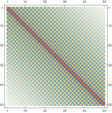
And now if we visualize this with H1 and H2 being odd-looking matrices which arise in this context:

 H1=Table[(1/2)(-1)^(i-j)If[i==j, π^2/3, 2/(i-j)^2], {i, 50}, {j, 50}];
H2=Table[((-1)^(i-j)/(2*(.05)^2))If[i==j, π^2/3, 2/(i-j)^2], {i, 75}, {j, 75}];
H1//MatrixPlot

We can directly construct H in a the standard fashion:

 H = 
  KroneckerProduct[H1, IdentityMatrix[Length@H2]] + 
    KroneckerProduct[IdentityMatrix[Length@H1], H2];//AbsoluteTiming//First

 4.523075`

It takes a while and we see it has a large memory footprint:

 H // ByteCount

 340260728

But if we visualize it we see it's most zeros:

 H // MatrixPlot

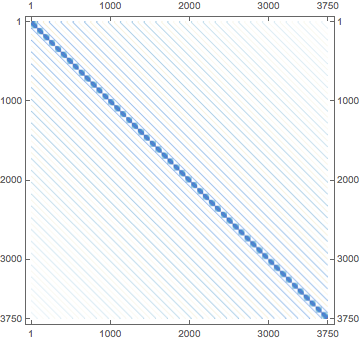
If we build it instead use SparseArray nothing will be done with that vast field of zeros, so it'll be faster and less memory intensive:

 HS = 
  KroneckerProduct[H1, IdentityMatrix[Length@H2, SparseArray]] + 
    KroneckerProduct[IdentityMatrix[Length@H1, SparseArray], H2];//AbsoluteTiming//First
HS//ByteCount

 0.118826`

 11191512

And even better, when we ask for its smallest 5 Eigenvalues these will be computed faster, and increasingly so with matrix size:

 Eigenvalues[H, -5]//AbsoluteTiming
Eigenvalues[HS, -5]//AbsoluteTiming

 {4.943048`,{0.3917953580905429`,0.3745580141408224`,0.3611510903074643`,0.35157483336542145`,0.34582905618130677`}}

 {3.733548`,{0.39179535809072363`,0.37455801414116613`,0.3611510903079675`,0.35157483336567635`,0.34582905618161475`}}